Part 1: Introduction to Purrr
Hello and welcome to the tutorial on Lists and Iterations with Purrr. Purrr is a tidyverse package that makes iterating over lists easier, more efficient, and more human readable compared to the base R functions. In the first section, we will learn the principal functions of purrr that will allow us to iterate over lists, how to troubleshoot lists, and dive into some more complex examples utilizing other tidyverse principals. In the second section of this tutorial, we will dive into more advanced topics including: lambda functions, partials, and predicate functions that will allow us to write cleaner code. Let’s begin!
#load required libraries
library(tidyverse)
library(repurrrsive)

#load sw_species dataset from repurrrsive
data("sw_species")

#examine the first element in sw_species
glimpse(sw_species[[2]])
## List of 15
##  $ name            : chr "Yoda's species"
##  $ classification  : chr "mammal"
##  $ designation     : chr "sentient"
##  $ average_height  : chr "66"
##  $ skin_colors     : chr "green, yellow"
##  $ hair_colors     : chr "brown, white"
##  $ eye_colors      : chr "brown, green, yellow"
##  $ average_lifespan: chr "900"
##  $ homeworld       : chr "http://swapi.co/api/planets/28/"
##  $ language        : chr "Galactic basic"
##  $ people          : chr "http://swapi.co/api/people/20/"
##  $ films           : chr [1:5] "http://swapi.co/api/films/5/" "http://swapi.co/api/films/4/" "http://swapi.co/api/films/6/" "http://swapi.co/api/films/3/" ...
##  $ created         : chr "2014-12-15T12:27:22.877000Z"
##  $ edited          : chr "2014-12-20T21:36:42.148000Z"
##  $ url             : chr "http://swapi.co/api/species/6/"
As shown above, we can use double brackets to subset an item or element in a list. In the case of the sw_species list, the second element corresponds to another list composed of information for Yoda’s species.
Another way to subset a list is by name using the $ followed by the list name, similar to how we subset dataframes. However, the sw_species list is unnamed.
#Get the names of the list elements
names(sw_species)
## NULL
Mapping
Our first task will be to apply names to each element using the $name subelement from each species sublist. One way to do this is by going through each list individually.
#get the name element from the first list in sw_species
(names(sw_species)[[1]] <- sw_species[[1]]$name)
## [1] "Hutt"
#examines the names of the sw_species once again
names(sw_species)
##  [1] "Hutt" NA     NA     NA     NA     NA     NA     NA     NA     NA
## [11] NA     NA     NA     NA     NA     NA     NA     NA     NA     NA
## [21] NA     NA     NA     NA     NA     NA     NA     NA     NA     NA
## [31] NA     NA     NA     NA     NA     NA     NA
This is painstakingly tedious and inefficent. One could use a for loop to do this, but there’s an even better way.
Purrr has a map function which works similarly to the base R apply functions. Map takes a .x argument - a vector or list, and a .f argument - a function. Map acts as a loop iterating the function over each element in the list. Let’s utilize map and the set_names function to give the sw_species dataset names.
First, we’ll create a list of species names. Map is useful in that the .f argument can be used to subset an element of the list as so:
#create a vector of names of the species
species_names <- map(sw_species, "name")
Now we’ll apply the species names to the sw_species list.
sw_species <- set_names(sw_species, species_names)

#examine the names of sw_species
names(sw_species)
##  [1] "Hutt"           "Yoda's species" "Trandoshan"     "Mon Calamari"
##  [5] "Ewok"           "Sullustan"      "Neimodian"      "Gungan"
##  [9] "Toydarian"      "Dug"            "Twi'lek"        "Aleena"
## [13] "Vulptereen"     "Xexto"          "Toong"          "Cerean"
## [17] "Nautolan"       "Zabrak"         "Tholothian"     "Iktotchi"
## [21] "Quermian"       "Kel Dor"        "Chagrian"       "Geonosian"
## [25] "Mirialan"       "Clawdite"       "Besalisk"       "Kaminoan"
## [29] "Skakoan"        "Muun"           "Togruta"        "Kaleesh"
## [33] "Pau'an"         "Wookiee"        "Droid"          "Human"
## [37] "Rodian"
#subset one of the lists using the $listelementname
sw_species$Ewok %>%
  simplify()
##                             name                   classification
##                           "Ewok"                         "mammal"
##                      designation                   average_height
##                       "sentient"                            "100"
##                      skin_colors                      hair_colors
##                          "brown"            "white, brown, black"
##                       eye_colors                 average_lifespan
##                  "orange, brown"                        "unknown"
##                        homeworld                         language
## "http://swapi.co/api/planets/7/"                        "Ewokese"
##                           people                            films
## "http://swapi.co/api/people/30/"   "http://swapi.co/api/films/3/"
##                          created                           edited
##    "2014-12-18T11:22:00.285000Z"    "2014-12-20T21:36:42.155000Z"
##                              url
## "http://swapi.co/api/species/9/"
By default, the map function returns elements in the form of a list. However, there are various flavors of map which will return different outputs:
| map_* | output |
|---|---|
| map_chr() | character vector |
| map_lgl() | logical vector [T or F] |
| map_int() | integer vector |
| map_dbl() | double vector (numeric) |
| map_df() | as data frame |
As an example, let’s use the map_chr function to grab the $language element from each species list which will return a character vector of the languages. Then we will use this character vector to create a data frame linking the languages back to the names of each species.
In order to do so we need to clarify a few things first:
To specify how the list is used in the function, use the argument .x to denote where the list element goes inside the function. When you want to use .x to show where the element goes in the function, you need to put a ~ in front of the function in the second argument of map().
data.frame(culture = map_chr(sw_species, ~.x$language)) %>%
  rownames_to_column(var = "character") %>%
  head(10)
##         character        culture
## 1            Hutt        Huttese
## 2  Yoda's species Galactic basic
## 3      Trandoshan           Dosh
## 4    Mon Calamari Mon Calamarian
## 5            Ewok        Ewokese
## 6       Sullustan      Sullutese
## 7       Neimodian      Neimoidia
## 8          Gungan   Gungan basic
## 9       Toydarian      Toydarian
## 10            Dug         Dugese
More Complex Operations
Piping
In the examples above, we saw that it is possible to using piping with the map function. The pipe allows us to streamline our code and makes it more human readable. Here’s another example.
#create a numeric list
(numlist <- list(c(1:10), c(11:20), c(21:30)))
## [[1]]
##  [1]  1  2  3  4  5  6  7  8  9 10
##
## [[2]]
##  [1] 11 12 13 14 15 16 17 18 19 20
##
## [[3]]
##  [1] 21 22 23 24 25 26 27 28 29 30
#use pipes to perform multiple operations
numlist %>%
  map(~.x %>%
      sum %>%
      sqrt %>%
      sin)
## [[1]]
## [1] 0.9056937
##
## [[2]]
## [1] -0.1162079
##
## [[3]]
## [1] -0.2578112
Simple mathematical operations are just the tip of the iceberg to what is possible. In this example, we’ll create some simulated data for housing around the bay area.
#create a list of areas
area <- list("San Francisco", "Oakland", "San Jose")

#create a list of dataframes with simulated housing data for each area
housing_list <- map(area,
                  ~data.frame(area = .x,
                              price = rnorm(mean = 800000,
                                            n = 100,
                                            sd = 800000/2.5),
                              sq_ft = rnorm(mean = 1200,
                                             n = 100,
                                             sd = 1200/4)
                  )
)

#examine a portion of the simulated data
map(.x = housing_list, .f = ~.x %>% head)
## [[1]]
##            area    price     sq_ft
## 1 San Francisco 436846.6 1304.4513
## 2 San Francisco 220175.2  934.5941
## 3 San Francisco 479857.4 1323.9702
## 4 San Francisco 956379.4 1487.9882
## 5 San Francisco 394394.7 1051.3588
## 6 San Francisco 746208.5  543.3655
##
## [[2]]
##      area     price     sq_ft
## 1 Oakland  795704.2 1350.4617
## 2 Oakland  800444.6 1072.7275
## 3 Oakland  528976.2 1216.5846
## 4 Oakland  661947.1 1269.7766
## 5 Oakland 1467022.9  948.1095
## 6 Oakland  542950.2 1389.0760
##
## [[3]]
##       area     price     sq_ft
## 1 San Jose  674574.3 1313.2285
## 2 San Jose 1288031.5  853.7149
## 3 San Jose  625760.2 1093.7647
## 4 San Jose 1546869.2  983.3692
## 5 San Jose 1401423.5 1488.4967
## 6 San Jose  772236.3 1150.3756
Now that we have the data let’s model each area using the map function.
#model the data using pipes and the map function
#notice that model function AND the summary function fall within the .f argument of the map function
housing_list %>%
  map(.f = ~.x %>% lm(price ~ sq_ft, data = .) %>% summary)
## [[1]]
##
## Call:
## lm(formula = price ~ sq_ft, data = .)
##
## Residuals:
##     Min      1Q  Median      3Q     Max
## -572842 -177694  -14188  173541  762638
##
## Coefficients:
##              Estimate Std. Error t value Pr(>|t|)
## (Intercept) 790896.07  140908.27   5.613 1.85e-07 ***
## sq_ft            2.27     111.29   0.020    0.984
## ---
## Signif. codes:  0 '***' 0.001 '**' 0.01 '*' 0.05 '.' 0.1 ' ' 1
##
## Residual standard error: 272000 on 98 degrees of freedom
## Multiple R-squared:  4.244e-06,	Adjusted R-squared:  -0.0102
## F-statistic: 0.0004159 on 1 and 98 DF,  p-value: 0.9838
##
##
## [[2]]
##
## Call:
## lm(formula = price ~ sq_ft, data = .)
##
## Residuals:
##     Min      1Q  Median      3Q     Max
## -801841 -216108  -26790  246719  801744
##
## Coefficients:
##             Estimate Std. Error t value Pr(>|t|)
## (Intercept) 927962.6   129172.6   7.184 1.34e-10 ***
## sq_ft         -101.4      103.8  -0.977    0.331
## ---
## Signif. codes:  0 '***' 0.001 '**' 0.01 '*' 0.05 '.' 0.1 ' ' 1
##
## Residual standard error: 312400 on 98 degrees of freedom
## Multiple R-squared:  0.009653,	Adjusted R-squared:  -0.0004522
## F-statistic: 0.9553 on 1 and 98 DF,  p-value: 0.3308
##
##
## [[3]]
##
## Call:
## lm(formula = price ~ sq_ft, data = .)
##
## Residuals:
##     Min      1Q  Median      3Q     Max
## -707082 -230878  -16980  210823  720399
##
## Coefficients:
##              Estimate Std. Error t value Pr(>|t|)
## (Intercept) 1164735.7   126499.3   9.207 6.35e-15 ***
## sq_ft          -248.6      101.4  -2.452    0.016 *
## ---
## Signif. codes:  0 '***' 0.001 '**' 0.01 '*' 0.05 '.' 0.1 ' ' 1
##
## Residual standard error: 307300 on 98 degrees of freedom
## Multiple R-squared:  0.05781,	Adjusted R-squared:  0.04819
## F-statistic: 6.013 on 1 and 98 DF,  p-value: 0.01597
Multiple Lists / Datasets
Purrr makes it easy to perform function(s) over multiple lists or datasets. For two lists, we can use map2 which requuires .x and .y as your list arguments. pmap handles more than two lists.
First let’s create a few lists.
#create a list of names
names_list <-map(sw_species, .f = ~.$name)

#create a list of lifespans
lifespan_list <- map(sw_species, .f = ~.$average_lifespan)

#create a list of languages
language_list <- map(sw_species, .f = ~.$language)
Now let’s create a dataframe using two of the lists.
#create a dataframe with the names and lifespan lists
map2_df(.x = names_list, .y = lifespan_list, .f = ~data.frame(names = .x, avg_lifespan = .y))
##             names avg_lifespan
## 1            Hutt         1000
## 2  Yoda's species          900
## 3      Trandoshan      unknown
## 4    Mon Calamari      unknown
## 5            Ewok      unknown
## 6       Sullustan      unknown
## 7       Neimodian      unknown
## 8          Gungan      unknown
## 9       Toydarian           91
## 10            Dug      unknown
## 11        Twi'lek      unknown
## 12         Aleena           79
## 13     Vulptereen      unknown
## 14          Xexto      unknown
## 15          Toong      unknown
## 16         Cerean      unknown
## 17       Nautolan           70
## 18         Zabrak      unknown
## 19     Tholothian      unknown
## 20       Iktotchi      unknown
## 21       Quermian           86
## 22        Kel Dor           70
## 23       Chagrian      unknown
## 24      Geonosian      unknown
## 25       Mirialan      unknown
## 26       Clawdite           70
## 27       Besalisk           75
## 28       Kaminoan           80
## 29        Skakoan      unknown
## 30           Muun          100
## 31        Togruta           94
## 32        Kaleesh           80
## 33         Pau'an          700
## 34        Wookiee          400
## 35          Droid   indefinite
## 36          Human          120
## 37         Rodian      unknown
pmap works a little differently. First, we need to create a master list, a list of lists so-to-speak.
#create a master list
species_info_list <- list(names = names_list, avg_lifespan = lifespan_list, language = language_list)

pmap_df(.l = species_info_list, .f = function(names, avg_lifespan, language) data.frame(names = names, avg_lifespan = avg_lifespan, language = language))
##             names avg_lifespan       language
## 1            Hutt         1000        Huttese
## 2  Yoda's species          900 Galactic basic
## 3      Trandoshan      unknown           Dosh
## 4    Mon Calamari      unknown Mon Calamarian
## 5            Ewok      unknown        Ewokese
## 6       Sullustan      unknown      Sullutese
## 7       Neimodian      unknown      Neimoidia
## 8          Gungan      unknown   Gungan basic
## 9       Toydarian           91      Toydarian
## 10            Dug      unknown         Dugese
## 11        Twi'lek      unknown       Twi'leki
## 12         Aleena           79         Aleena
## 13     Vulptereen      unknown     vulpterish
## 14          Xexto      unknown        Xextese
## 15          Toong      unknown         Tundan
## 16         Cerean      unknown         Cerean
## 17       Nautolan           70        Nautila
## 18         Zabrak      unknown        Zabraki
## 19     Tholothian      unknown        unknown
## 20       Iktotchi      unknown     Iktotchese
## 21       Quermian           86       Quermian
## 22        Kel Dor           70        Kel Dor
## 23       Chagrian      unknown        Chagria
## 24      Geonosian      unknown      Geonosian
## 25       Mirialan      unknown       Mirialan
## 26       Clawdite           70       Clawdite
## 27       Besalisk           75       besalisk
## 28       Kaminoan           80       Kaminoan
## 29        Skakoan      unknown        Skakoan
## 30           Muun          100           Muun
## 31        Togruta           94        Togruti
## 32        Kaleesh           80        Kaleesh
## 33         Pau'an          700        Utapese
## 34        Wookiee          400     Shyriiwook
## 35          Droid   indefinite            n/a
## 36          Human          120 Galactic Basic
## 37         Rodian      unknown Galactic Basic
Here’s another example using pmap. Notice that we don’t need to use the function argument to define the list elements.
a <- list(1:100)
b <- list(rnorm(10, 25, 2))
c <- list(seq(from = 10, to = 1000, by = 3))

pmap(.l = list(a,b,c), .f = sum)
## [[1]]
## [1] 172458.8
Troubleshooting Lists
Safely
safely runs through a list returning result and error components making it easier to pinpoint issues.
#create a list 'foo'
foo <- list(3, -10, Inf, "a")

#use map function on foo
map(foo, log)
## Error in log(x = x, base = base): non-numeric argument to mathematical function
As you see, we get an error somewhere in the list. We know that we can’t take the log of “a”, but what if our list was much larger? It would be very difficult to troubleshoot. This is exactly what safely is designed for.
#use safely with map function
map(foo, .f = safely(log, otherwise = NA_real_))
## [[1]]
## [[1]]$result
## [1] 1.098612
##
## [[1]]$error
## NULL
##
##
## [[2]]
## [[2]]$result
## [1] NaN
##
## [[2]]$error
## NULL
##
##
## [[3]]
## [[3]]$result
## [1] Inf
##
## [[3]]$error
## NULL
##
##
## [[4]]
## [[4]]$result
## [1] NA
##
## [[4]]$error
## <simpleError in log(x = x, base = base): non-numeric argument to mathematical function>
It is useful to use the transpose function in conjunction with troubleshooting functions such as safely to convert a list of pairs into a pair of lists for easier comprehension.
#use transpose after function to split out results and errors
foo %>%
  map(safely(log, otherwise = NA_real_)) %>%
  transpose()
## $result
## $result[[1]]
## [1] 1.098612
##
## $result[[2]]
## [1] NaN
##
## $result[[3]]
## [1] Inf
##
## $result[[4]]
## [1] NA
##
##
## $error
## $error[[1]]
## NULL
##
## $error[[2]]
## NULL
##
## $error[[3]]
## NULL
##
## $error[[4]]
## <simpleError in log(x = x, base = base): non-numeric argument to mathematical function>
Possibly
Once we have figured out where the errors exist, we can replace safely with possibly to implement the change (e.g. inserting an ‘NA’ where all errors occur) without returning the error message.
#use possibly to output list without errors
foo %>%
  map_dbl(possibly(log, otherwise = NA_real_))
## [1] 1.098612 NaN Inf NA
Let’s take a look at one more example using the Star Wars Species data we’re already familiar with. Within the species list, there is a height subelement indicating the height of each species in centimeters. Let’s isolate this element and convertthe measurement to feet.
#extract the height subelement
sw_species %>%
  map(~.$average_height) %>%
  map_dbl(as.numeric) %>%
  map_dbl(~.x * 0.0328084, otherwise = NA_real_)
##           Hutt Yoda's species     Trandoshan   Mon Calamari           Ewok
##       9.842520       2.165354       6.561680       5.249344       3.280840
##      Sullustan      Neimodian         Gungan      Toydarian            Dug
##       5.905512       5.905512       6.233596       3.937008       3.280840
##        Twi'lek         Aleena     Vulptereen          Xexto          Toong
##       6.561680       2.624672       3.280840       4.101050       6.561680
##         Cerean       Nautolan         Zabrak     Tholothian       Iktotchi
##       6.561680       5.905512       5.905512             NA       5.905512
##       Quermian        Kel Dor       Chagrian      Geonosian       Mirialan
##       7.874016       5.905512       6.233596       5.839895       5.905512
##       Clawdite       Besalisk       Kaminoan        Skakoan           Muun
##       5.905512       5.839895       7.217848             NA       6.233596
##        Togruta        Kaleesh         Pau'an        Wookiee          Droid
##       5.905512       5.577428       6.233596       6.889764             NA
##          Human         Rodian
##       5.905512       5.577428
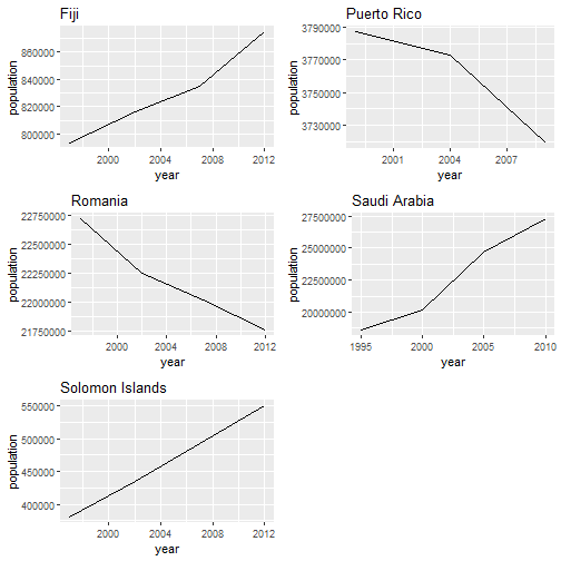
Walk
The walk function makes list outputs more human readable. It calls the function (.f) for its ‘side-effect’ and returns the input (.x) removing all the unnecessary list bracketing.
In the example below we’ll use the population dataset from the tidyr package to plot year vs. population for a selection of countries.
library(gridExtra) #for arranging plots

#select a random sample of countries
(countries <- unique(population$country) %>%
  sample(size = 5))
## [1] "Romania"         "Puerto Rico"     "Solomon Islands" "Fiji"
## [5] "Saudi Arabia"
plots <- population %>%
  filter(country == countries) %>% # filter only countries of interest
  split(.$country) %>% # split the data by country
  map2(.x = .,
       .y = names(.),
       .f = ~ggplot(.x, aes(x = year, y = population)) +
         geom_line() +
         labs(title = .y))

plots %>%
  walk(grid.arrange(grobs = .))
## Error: Can't convert a `gtable` object to function
Problem Solving
Now that we have some experience working with various functions in R, let’s put our new found skills to the test by solving some problems. The gh_users dataset is also from the repurrrsive package and provides some data on github users.
First, let’s take a look at the dataset.
#summarize the dataset
summary(gh_users)
##      Length Class  Mode
## [1,] 30     -none- list
## [2,] 30     -none- list
## [3,] 30     -none- list
## [4,] 30     -none- list
## [5,] 30     -none- list
## [6,] 30     -none- list
#determine whether the dataset is named
names(gh_users)
## NULL
The gh_users daatset is comprised of 6 lists each comprised of 30 elements. We also know that the lists do not contain names. Let’s take a look at the elements from the first list to see what kind of information is included.
#exmaine the structure of the first list
str(gh_users[[1]])
## List of 30
##  $ login              : chr "gaborcsardi"
##  $ id                 : int 660288
##  $ avatar_url         : chr "https://avatars.githubusercontent.com/u/660288?v=3"
##  $ gravatar_id        : chr ""
##  $ url                : chr "https://api.github.com/users/gaborcsardi"
##  $ html_url           : chr "https://github.com/gaborcsardi"
##  $ followers_url      : chr "https://api.github.com/users/gaborcsardi/followers"
##  $ following_url      : chr "https://api.github.com/users/gaborcsardi/following{/other_user}"
##  $ gists_url          : chr "https://api.github.com/users/gaborcsardi/gists{/gist_id}"
##  $ starred_url        : chr "https://api.github.com/users/gaborcsardi/starred{/owner}{/repo}"
##  $ subscriptions_url  : chr "https://api.github.com/users/gaborcsardi/subscriptions"
##  $ organizations_url  : chr "https://api.github.com/users/gaborcsardi/orgs"
##  $ repos_url          : chr "https://api.github.com/users/gaborcsardi/repos"
##  $ events_url         : chr "https://api.github.com/users/gaborcsardi/events{/privacy}"
##  $ received_events_url: chr "https://api.github.com/users/gaborcsardi/received_events"
##  $ type               : chr "User"
##  $ site_admin         : logi FALSE
##  $ name               : chr "Gábor Csárdi"
##  $ company            : chr "Mango Solutions, @MangoTheCat "
##  $ blog               : chr "http://gaborcsardi.org"
##  $ location           : chr "Chippenham, UK"
##  $ email              : chr "csardi.gabor@gmail.com"
##  $ hireable           : NULL
##  $ bio                : NULL
##  $ public_repos       : int 52
##  $ public_gists       : int 6
##  $ followers          : int 303
##  $ following          : int 22
##  $ created_at         : chr "2011-03-09T17:29:25Z"
##  $ updated_at         : chr "2016-10-11T11:05:06Z"
Now, let’s determine which of the users has the most public repositories.
map_int(gh_users, ~.$public_repos) %>% #pull out the # of public repositories
  set_names(map_chr(gh_users, ~.$name)) %>% #assign names to each list element
  sort(decreasing = T) #sort the data
## Jennifer (Jenny) Bryan       Thomas J. Leeper                Jeff L.
##                    168                     99                     67
##           Gábor Csárdi          Maëlle Salmon            Julia Silge
##                     52                     31                     26
And there you have it. Jennifer Bryan has the most repositories with a whopping 168.
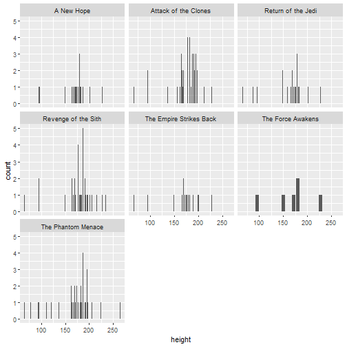
And now for another example. Let’s use the sw_films and sw_people data. Here, we want to join the two datasets so we can plot the height distributions of the characters according to the movies they appear in.
# Turn data into correct dataframe format
film_by_character <- tibble(filmtitle = map_chr(sw_films, ~.$title)) %>%
    mutate(filmtitle, characters = map(sw_films, ~.$characters)) %>%
    unnest()

# Pull out elements from sw_people
sw_characters <- map_df(sw_people, `[`, c("height", "mass", "name", "url"))

# Join the two new objects
character_data <- inner_join(film_by_character, sw_characters, by = c("characters" = "url")) %>%
    # Make sure the columns are numbers
    mutate(height = as.numeric(height), mass = as.numeric(mass))

# Plot the heights, faceted by film title
ggplot(character_data, aes(x = height)) +
  geom_histogram(stat = "count") +
  facet_wrap(~ filmtitle)
Part 2
Now that we have a sense of how purrr uses the map to iterate over data, let’s look at other functions that will make it easier to write more complex code.
Mappers
A classical function is also known as a lambda or anonymous function because it is unnamed and created in the context of the iteration.
There are three main advantages to using mappers:
- concise
- easy to read
- reusable
Mappers take on a one-sided formula. We start with a ~ followed by the formula and a .x to refer to the list input we want to iterate over in the function. We can also use a single dot . or ..1 in place of .x.
Here’s an example using the list numlist we created earlier in the tutorial.
#examine the list 'numlist'
str(numlist)
## List of 3
##  $ : int [1:10] 1 2 3 4 5 6 7 8 9 10
##  $ : int [1:10] 11 12 13 14 15 16 17 18 19 20
##  $ : int [1:10] 21 22 23 24 25 26 27 28 29 30
#a simple map function
map(numlist, mean)
## [[1]]
## [1] 5.5
##
## [[2]]
## [1] 15.5
##
## [[3]]
## [1] 25.5
# mapper with .
map(numlist, ~ mean(.) + 2)
## [[1]]
## [1] 7.5
##
## [[2]]
## [1] 17.5
##
## [[3]]
## [1] 27.5
# mapper with ..1
map(numlist, ~ mean(..1) %>% sqrt)
## [[1]]
## [1] 2.345208
##
## [[2]]
## [1] 3.937004
##
## [[3]]
## [1] 5.049752
It is good practice to write a function for anything you have to do more than twice.
Let’s suppose the list numlist is temeprature readings in celsius and we want to convert them to farenheit.
# create a function to convert celsius to farnehit
c_to_f <- function(x){
  (x * 9/5) + 32
}

#iterate over numlist with c_to_f function
map(.x = numlist, .f = c_to_f)
## [[1]]
##  [1] 33.8 35.6 37.4 39.2 41.0 42.8 44.6 46.4 48.2 50.0
##
## [[2]]
##  [1] 51.8 53.6 55.4 57.2 59.0 60.8 62.6 64.4 66.2 68.0
##
## [[3]]
##  [1] 69.8 71.6 73.4 75.2 77.0 78.8 80.6 82.4 84.2 86.0
We can also create a mapper using the as_mapper function which requires less code.
#create c_to_f function using as_mapper
c_to_f <- as_mapper(~ (.x * 9/5) + 32)

#iterate over numlist with mapper function
map(.x = numlist, .f = c_to_f)
## [[1]]
##  [1] 33.8 35.6 37.4 39.2 41.0 42.8 44.6 46.4 48.2 50.0
##
## [[2]]
##  [1] 51.8 53.6 55.4 57.2 59.0 60.8 62.6 64.4 66.2 68.0
##
## [[3]]
##  [1] 69.8 71.6 73.4 75.2 77.0 78.8 80.6 82.4 84.2 86.0
Cleaning Data with Mappers & Predicates
80% of data science is cleaning the data. It’s not glamarous, but it’s the truth.
When dealing with lists, there are a few useful functions we can utilize in conjunction with mappers to help us clean up the data. We’ll refer to these as predicates.
Predicate functions are those which test a condition and return either True or False. is.numeric is an example of a predicate function; so are the >, <, and == operators.
On the other hand, predicate functionals take an object and a predicate function and return some value. keep, discard, every, and some are examples of predicate functionals available in purrr.
Keep & Discard
As the name suggests keep is a logical function which will return any data in which the condition is met. Discard will do the opposite.
#examine foo
foo
## [[1]]
## [1] 3
##
## [[2]]
## [1] -10
##
## [[3]]
## [1] Inf
##
## [[4]]
## [1] "a"
#keep character elements
keep(foo, is.character)
## [[1]]
## [1] "a"
Let’s take a look at a more complex example. We’ll use the sw_species list again. Here, we want to discard any species whose lifespan is unknown.
discard(sw_species, ~.x$average_lifespan == 'unknown') %>%
  map("average_lifespan") %>%
  simplify()
##           Hutt Yoda's species      Toydarian         Aleena       Nautolan
##         "1000"          "900"           "91"           "79"           "70"
##       Quermian        Kel Dor       Clawdite       Besalisk       Kaminoan
##           "86"           "70"           "70"           "75"           "80"
##           Muun        Togruta        Kaleesh         Pau'an        Wookiee
##          "100"           "94"           "80"          "700"          "400"
##          Droid          Human
##   "indefinite"          "120"
Predicate functions work well in conjunction with mappers as in the following example:
#examine numlist
numlist
## [[1]]
##  [1]  1  2  3  4  5  6  7  8  9 10
##
## [[2]]
##  [1] 11 12 13 14 15 16 17 18 19 20
##
## [[3]]
##  [1] 21 22 23 24 25 26 27 28 29 30
#mapper for divisible by three
divisible_by_three <- as_mapper(~.x %% 3 == 0)

#map over numlist applying keep and mapper function
map(numlist, ~keep(.x, divisible_by_three))
## [[1]]
## [1] 3 6 9
##
## [[2]]
## [1] 12 15 18
##
## [[3]]
## [1] 21 24 27 30
Writing cleaner code
As we’ve seen so far, purrr is a useful package for writing cleaner code and offers the following advantages:
- light - less code written overall
- readable - less repetition, focus on what’s being executed
- interpretable - code becomes more specific and easier to understand in the long run
- maintainable - easier to fix if errors arise
In the last section of this tutorial, we’ll look at a few more examples of how we can simplify what would otherwise be seemingly complex operations.
Compose & Partial
The compose function allows us to utilize multiple functions. The caveat is that functions are applied right to left within the function itself.
The partial function allows us to write a function in which we specify some of the arguments. This could be useful if we know we’ll be using a function repeatedly on different datasets where most of the arguments will remain the same.
We’ll take a look at the housing_list data we created earlier in this tutorial. First, let’s summarize the data to see what we’re working with.
#summary of housing_list
map(housing_list, summary)
## [[1]]
##             area         price             sq_ft
##  San Francisco:100   Min.   : 220175   Min.   : 543.4
##                      1st Qu.: 615306   1st Qu.:1070.5
##                      Median : 780210   Median :1218.2
##                      Mean   : 793716   Mean   :1242.4
##                      3rd Qu.: 967906   3rd Qu.:1432.8
##                      Max.   :1556777   Max.   :1805.0
##
## [[2]]
##       area         price             sq_ft
##  Oakland:100   Min.   :  33256   Min.   : 565.1
##                1st Qu.: 599379   1st Qu.: 998.2
##                Median : 798434   Median :1209.4
##                Mean   : 805460   Mean   :1207.6
##                3rd Qu.:1048556   3rd Qu.:1427.1
##                Max.   :1618562   Max.   :2058.4
##
## [[3]]
##        area         price             sq_ft
##  San Jose:100   Min.   : 163670   Min.   : 541.6
##                 1st Qu.: 644449   1st Qu.: 984.7
##                 Median : 863856   Median :1171.0
##                 Mean   : 863834   Mean   :1210.3
##                 3rd Qu.:1073601   3rd Qu.:1424.4
##                 Max.   :1599627   Max.   :1906.4
It appears there are some houses with negative prices. We can’t have houses with negative sales prices, that just doesn’t make sense. Let’s create a partial function that discards these negative values.
#partial function to discard negatives
discard_negatives <- partial(discard, .p = ~.x < 0)
Unfortunately, I can’t use the function by itself because housing_list is a list of dataframes and the discard function, along with other predicate functions, only works on lists in an elementwise fashion. In the following example, we’ll workaround this issue using two useful functions: transpose and flatten.
transpose will turn the list ‘inside-out converting the dataframes into lists. This will allow us to map over the list with the other functions we’ve composed. Finally, we’ll use flatten to make the output more readable.
#compose a function that will flatten the data,
#discard the negatives,
#and finally takes the mean of each list
get_means <- compose(round, mean, discard_negatives)

housing_list %>%
  set_names(area) %>%
  transpose() %>%
  map(. %>% map(get_means)) %>%
  map(flatten_df)
## $area
## # A tibble: 1 x 3
##   `San Francisco` Oakland `San Jose`
##             <dbl>   <dbl>      <dbl>
## 1              NA      NA         NA
##
## $price
## # A tibble: 1 x 3
##   `San Francisco` Oakland `San Jose`
##             <dbl>   <dbl>      <dbl>
## 1          793716  805460     863834
##
## $sq_ft
## # A tibble: 1 x 3
##   `San Francisco` Oakland `San Jose`
##             <dbl>   <dbl>      <dbl>
## 1            1242    1208       1210
Putting It All Together
By know, you should have a solid understanding of how the purrr package makes writing code much more efficient. From iterating over lists, to troubleshooting,stringing together functions and cleaning data,there’s little purrr can’t handle.
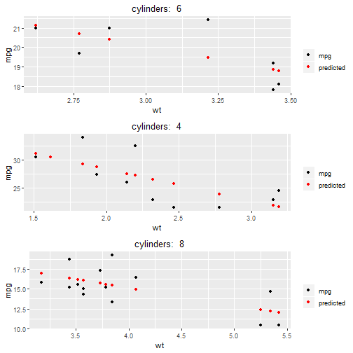
In this final example, we’ll use some of what we’ve learned to split up a dataset using grouping and nesting, create multiple models, and plot the data.
library(modelr)

#compose the function
group_nest <- compose(nest, group_by)

nested_data <- group_nest(mtcars, cyl)

model1 <- function(x){
  lm(mpg ~ wt, data = x)
}


nested_data %>%
  mutate(model = map(data, model1)) %>%
  mutate(pred = map2(data, model, add_predictions)) %>%
  map2(.x = .$pred,
       .y = .$cyl,
       .f = ~ggplot(.x, aes(x = wt))+
         geom_point(aes(y = mpg, colour = "mpg"))+
         geom_point(aes(y = pred, colour = "predicted")) +
         scale_colour_manual("", values = c("mpg"= "black", "predicted" = "red")) +
         labs(title = paste("cylinders: ", .y)) +
         theme(plot.title = element_text(hjust = .5))) %>%
  walk(grid.arrange(grobs = .))
## Error: Can't convert a `gtable` object to function